When a user adds rows or column headings in the worksheet, it is not visible while scrolling up and down the worksheet. MS Excel offers a smart solution for this with freezing panes. Freezing panes simply helps in keeping the heading visible while scrolling through the worksheet.

Using Freeze Panes

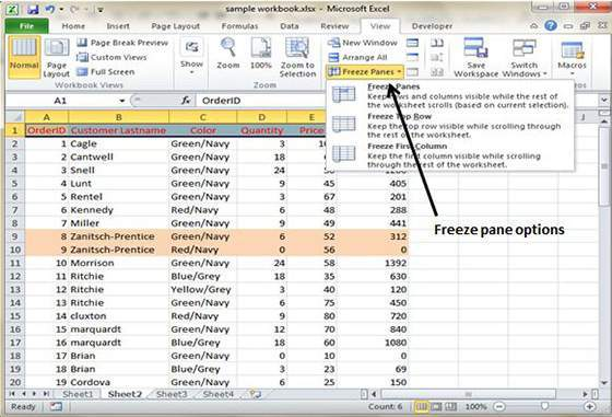
• Select the first row or column or row Below which you like to freeze. Users can even select the Column right to area that they want to freeze.
• Choose View tab followed by Freeze Panes.
• Then select from the variety of suitable option:
  • Freeze Panels – It freezes the area of cells.
  • Freeze Top Row – It freezes the first row of worksheet.
  • Freeze First Column – It freezes the first Column of worksheet.

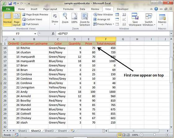
If you select the Freeze top, then you find that first row appears at the top while scrolling, like this.

Unfreeze Panes

In order to unfreeze Panes, simply choose View Tab and click on Unfreeze Panes.