MS Excel offers the feature of data filtering wherein worksheet display only those rows which meets the certain conditions set by the user. The other ‘rows’ which doesn’t satisfy the condition simply remains hidden from the view.

Here is an example where earlier stored data is utilized. Here we are trying to see the data relating to Shoe Size 36. This can be done easily by using the filter. Follow these smart steps below:

• Place the cursor on the Header Row
• Now choose the Data Tab, followed by Filter in order to set filter.

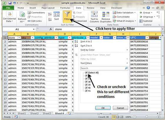
• Click on the drop down area in the Area Row Header. Remove the check mark from the Select All and it will help in unselecting everything.
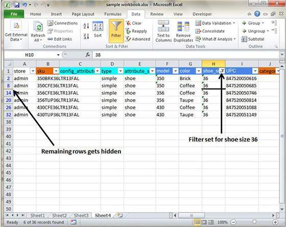
• We are looking to for the Size 36, therefore select the check mark on the Size 36. This will result in filtering the data and it will only display the data of Size 36.
• You will find some of the rows are missing. These rows are simply hidden from the view as they fail to meet the condition.
• Now the drop down arrow in the Area column will show a different graphic. An icon will appear in the worksheet columns name area, which will indicate that this particular column has been filtered.

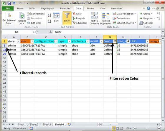
Using Multiple Filters

You can make use of multiple filters in order to meet multiple conditions in the worksheet. As with the given example, suppose you wish to have the data filtered as per the color of ‘coffee’ after filtering it by size 36, then it can be done by using the multiple filters.

First, set the filter for the Shoe size like before hen choose the Color column and set the filter for the color.