How To Create Pivot Charts In MS Excel 2010
Pivot charts are widely used charts in the worksheet, which brings a graphical representation of the data summary displayed in the pivot table. Excel offers a great flexibility to the users by allowing them to create a pivot table and a pivot chart at the same time. One can even create a pivot chart without creating a pivot table, which is added benefit.
Pivot charts can be accessed under the Insert Tab, followed by PivotTable dropdown and finally the PivotChart.
Pivot Chart Example
An example will help in understanding how to create a pivot chart in Excel 2010. Assume you are required to showcase the huge data of voters in a summarized view in a form of the charts, then you can make use of the Pivot chart. Go to the Insert Tab, followed by the PivotChart in order to insert a pivot table.
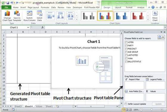
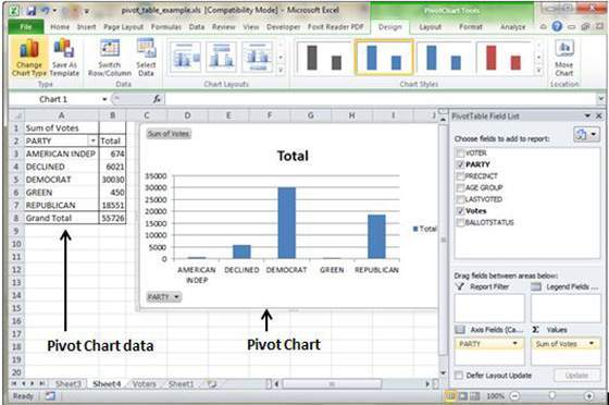
MS Excel will use the data right from this table. Users can even select the pivot chart location present either in the existing sheet or in some other sheet. Pivot chart will be created automatically by the MS Excel based on the data present in the pivot table. The resulting pivot will appear like the below-mentioned image.
Tags How To Create Pivot Charts In MS Excel 2010MS Excel Tutorial

You may also like...


Sorry - Comments are closed