MS Excel offers a Conditional Formatting feature that allows user to format a range of values.

Simply choose Home Tab, followed by Style Group and select Conditional Formatting dropdown.

Different conditional formatting options

• Highlight cell rules – It helps to highlight the cells in the cell selection on basis of certain values, texts, dates or other parameters.
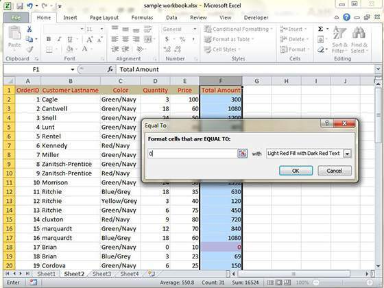
  For instance, if you have to find cell with Amount 0 and Mark them as red, then choose Range of cell, followed by Home Tab, Conditional Formatting Dropdown, Highlight Cell Rules and finally Equal To.

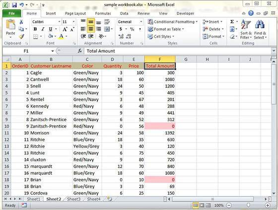
Once you give a click on OK, all the cells with zero value will be marked as red.

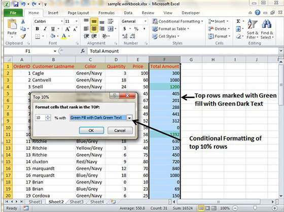
• Top/Bottom Rules – This will help in highlighting the top and bottom cells based on values, percentages and other parameters. For instance, if you have to highlight top 10% rows, use the Top/Bottom rules.

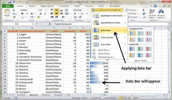
• Data Bars – It brings up a palette with different colors data bars applied to the cell selection for indicating their values relative to each other.
  This particular conditional formatting data Bars will appear in every cell.

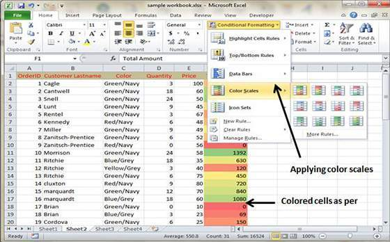
• Color Scales – It brings a palette with different three or two colored scales which when applied to the cell selection indicate vales relative to each other.

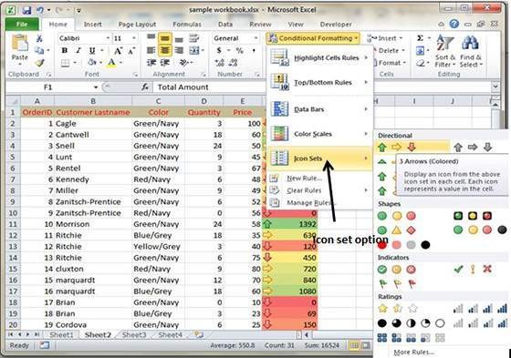
• Icon Sets – It brings a palette that shows different set of icons and gets applied to each cell.

• New Rule – It brings the New Formatting Rule dialog box where users can define custom conditional formatting rules for all the cell selection.
• Clear Rules – It helps in removing the conditional formatting for the cell selection.
• Manage Rules – It opens up the Conditional Formatting Rules Manager for editing or deleting particular rules.