How To Perform Cross Referencing In MS Excel 2010
Graphic Object in MS Excel
Over time, most of the users find themselves having huge amount of information spread across several different worksheets. It is very challenging and frustrating tasks to bring all these different data together in a single table for better understanding. MS Excel offers a very helpful feature called Vlookup function, which helps in this case.
VLOOKUP
VlookUp works by searching for the value in the vertical manner in the lookup table. VLOOKUP(lookup_value, table_array,col_index_num,range_lookup) has just four parameters which has to be filled with accurately.
- Lookup_value – It is the user input. VlookpUp function makes use of this value to perform the search.
- The table_array – It happens to be area of cell specifically in which the table is located.
- Col_index_num – It is the column of data which contains the answer you are searching for.
- Range_lookup – Here one has to enter either TRUE or False value. Setting it at TRUE will ensure that lookup function finds the closest match to the lookup_value. Setting it at FALSE will ensures that the vlookup function finds the exact match for the lookup_value elsewise it will return #N/A.
VLOOKUP Example
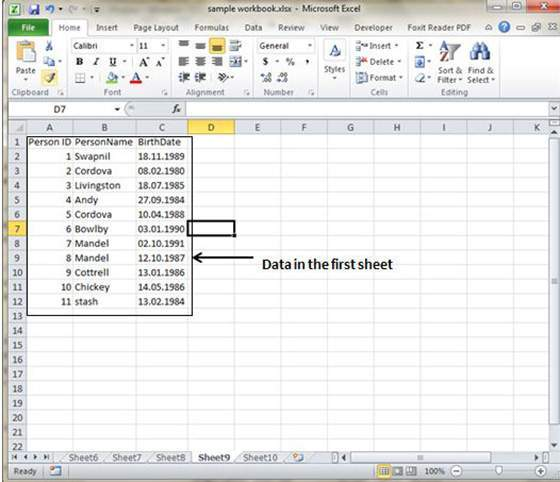
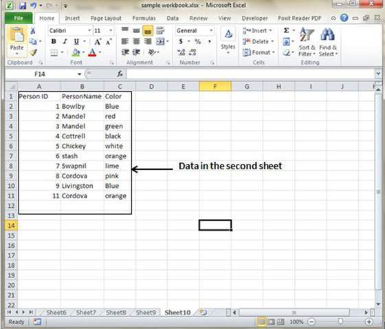
Here is a simple example of cross-referencing using two worksheets. Each of the worksheet here contains information related to the same group of people. The first worksheet contains information related to the date of birth while second contains the information on the favorite color.
Here, we will try to build a table that will show the person’s name along with their date of birth and their favorite color. Vlookup will be used to achieve this simple cross-referencing table.
The data present in the first worksheet.
The data present in the second worksheet.
In order to find the respective favorite color of the person from other sheet, we will use the vlookup function. In vloopup function, the first parameter is lookup value that can be set as person name. Second parameter is the table array, which will be set as the table present in the second sheet from B2 to C11. Third parameter is the Column Index num and it will be set as 2 as the color column is at 2 position in the table. The fourth parameter can be set at TRUE for returning partial match or at FALSE To return an exact match. Clicking on OK will allow the VLOOKUP function to calculate the colors and results will be displayed on the screen like below.
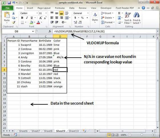
Now you can see in the above image that VLOOKUP has complete it search and displayed its result in the table form containing both the date of birth and the favorite color. It has also returned #N/A in certain where matches has not been found. Andy data is not present in the second worksheet hence it relative boxes shows #N/A.
Tags How To Perform Cross Referencing In MS Excel 2010MS Excel Tutorial

You may also like...


Sorry - Comments are closed